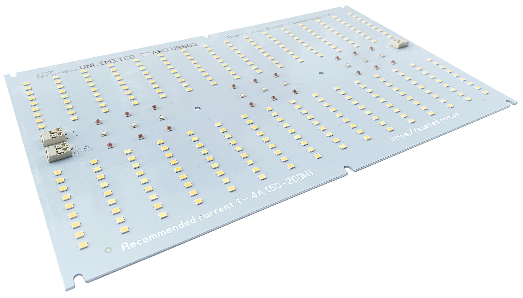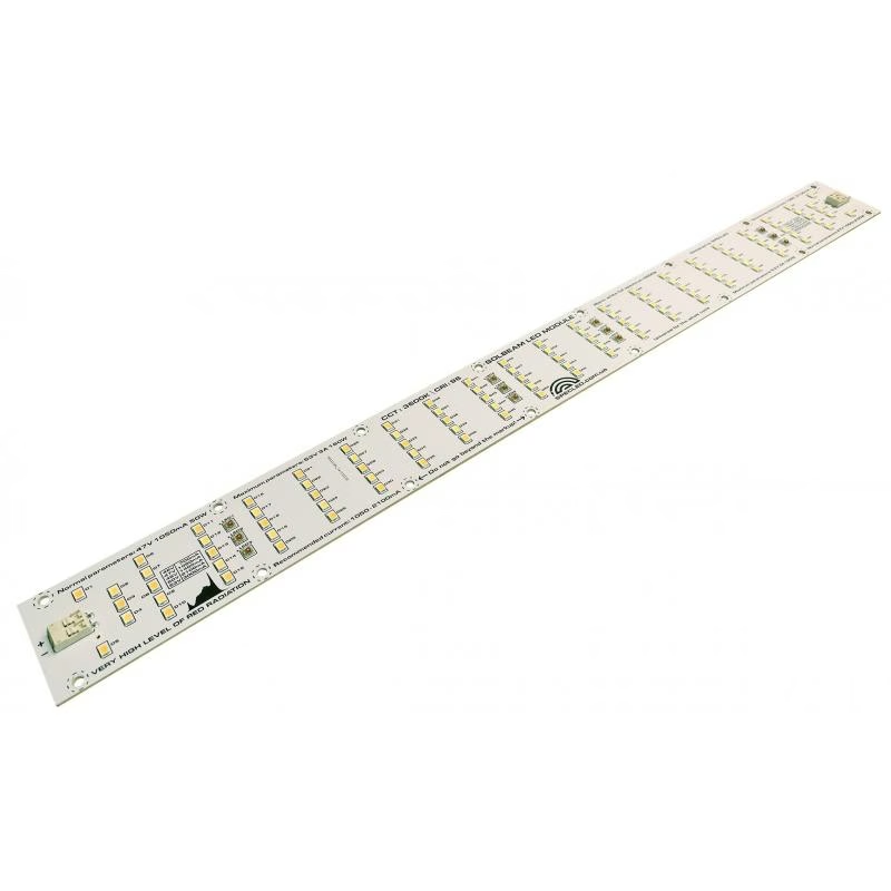
Every LED has a datasheet, and in the datasheet everything looks, if not perfect, then at least good. The problem is that a datasheet describes a diode, while the customer receives a luminaire. Between the two sit the driver, the operating current, the junction temperature, the particular bin from the batch, the board geometry, the heatsink, the real operating conditions. Every one of these pulls the actual numbers away from the tabulated ones, and never for the better.
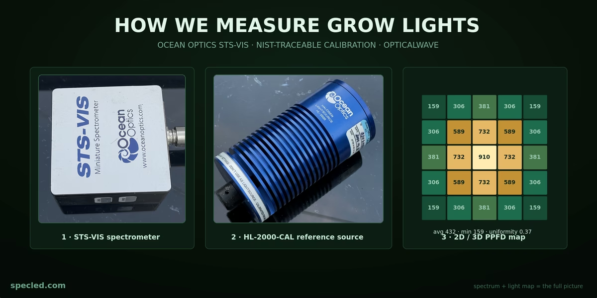
It follows that the only way to get a lamp's "live" characteristics is to measure them. And it is worth measuring not just the spectrum and the basic light parameters, but also building a 2D — better still, a 3D — light map. In essence, the spectrum tells you what kind of light you have, while the light map tells you where it lands and how much of it arrives. Below is the equipment and the software we use to do this.
Why we don't trust the LED datasheet
Let me say up front: manufacturers are not lying. Their numbers are simply obtained under laboratory conditions, while you switch the lamp on in a grow tent. On top of that, most LED manufacturers quote their parameters at a junction temperature of 25 °C, and that is unattainable with any real cooling system. Unless, of course, you live in Greenland.
Efficacy is the classic example. The table shows a handsome µmol/J↗ figure, but it was measured at a specific current and at a junction temperature you will almost never see in a real assembly. Drive the LED above its nominal current to squeeze more flux out of the same area and efficacy drops. Let the die overheat and it drops again, and the spectrum shifts along with it (that error is negligible, within 2–3 nm).
Then the arithmetic of the assembly kicks in. The datasheet has one diode; a module has a hundred, sitting side by side and warming each other like penguins in Antarctica. Add the driver with its own efficiency, add losses in the optics or the protective glass, add losses to reflection off the board and the heatsink.
The upshot is that the characteristics of a finished luminaire are not the characteristics of a diode multiplied by the number of diodes. They are a separate quantity, and it has to be measured separately, under real conditions, and only on a fully warmed-up lamp.
The Ocean Optics STS-VIS spectrometer
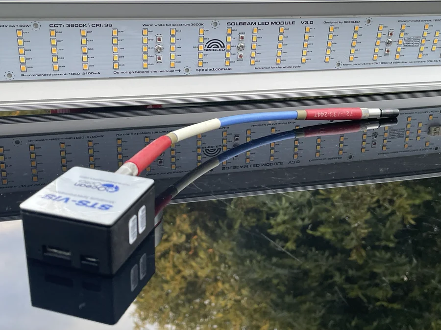
This is a compact visible-range spectrometer. Instruments like this are commonly called spectrophotometers, although strictly speaking measuring a source's own emission is spectroradiometry. It covers the entire PAR region, and that is enough for everything we need from a grow light or an individual LED.
Here is what we get out of it. First of all, the shape of the spectrum: exactly where the peaks sit, how broad they are, what happens in the dip between blue and red, how much energy goes into far-red. Everything else is then calculated from the spectrum: the share of each waveband, the blue-to-red ratio and, with an absolute calibration, the photon flux itself (PPFD↗).
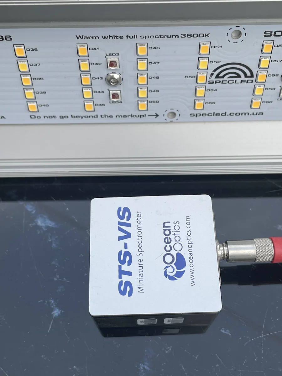
The light's path into the spectrometer: optical fiber and cosine corrector
The spectrometer itself is, crudely speaking, a box with a slit. Everything that happens before that slit determines what you end up measuring, and this is not the place to cut corners.
When I ordered the instrument, I went straight for a premium fiber optic cable with a 600 µm core and a CC-VIS/NIR cosine corrector. About the fiber, briefly: core area grows as the square of the diameter, so 600 µm collects roughly nine times more light than the common 200 µm. In practice that means shorter integration times and a cleaner signal in the weak parts of the spectrum — in far-red, in the ultraviolet, in the dip between the blue and red peaks. Which is precisely where good grow lights differ from mediocre ones.
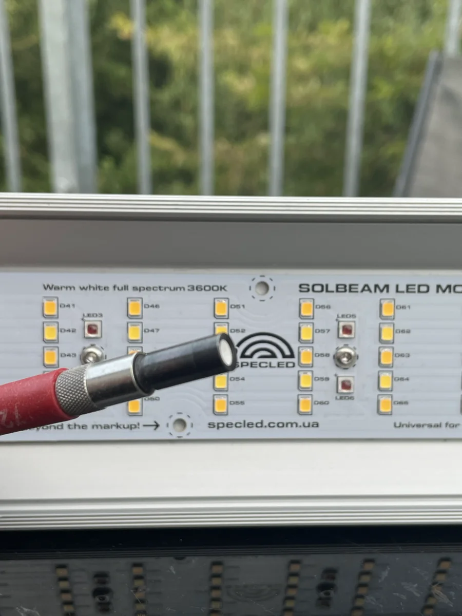
The cosine corrector is the part without which absolute measurements simply make no sense. A bare fiber sees a narrow cone of some twenty-five degrees: aim it slightly differently and you get a different number. A plant leaf works differently. It lies in a plane and receives light from the entire hemisphere above it: directly from the luminaire, from the neighbouring luminaire, reflected off the walls of the tent. The corrector makes the instrument collect light the same way.
CC-VIS/NIR cosine corrector specifications
| Parameter | Value |
|---|---|
| Diameter of active area | 3.9 mm |
| Diffusing material | quartz (200–2500 nm), ca. 1.5 mm thick |
| Dimensions | 6.5 mm diameter, 18 mm long |
| Sampling geometry | accepts light at/from 180° FOV |
| Connector | SMA 905 |
| Temperature | −30 °C … +100 °C |
Diameter of active area — 3.9 mm. The working "window" through which light is collected. The measurement is effectively a point measurement: when a light map is taken with a step of a few centimetres, a four-millimetre spot is a point, not an average over an area.
Diffuser — quartz (200–2500 nm), about 1.5 mm. Quartz specifically, not plastic. Quartz is transparent from the deep UV to the near IR, so it cuts off neither UV-A at 380 nm nor far-red at 730 nm — the two edges of the range that matter most in a horticultural spectrum. And it does not yellow under ultraviolet over time, unlike polymer diffusers.
Dimensions — 6.5 mm diameter, 18 mm long. The probe is small, so it neither shades the area nor distorts the very field it is measuring. It is also easy to move from cell to cell when taking a map.
Sampling geometry — 180° field of view. The most important line in the whole table. 180° is a full hemisphere, ±90° from the normal: the detector accepts everything arriving from above, right down to rays grazing almost parallel to the plane. And its response follows the cosine law — light arriving at angle θ is counted with a weight of cos θ. That is exactly how any horizontal surface receives light, whether a single leaf or the whole canopy. The measured value is therefore the irradiance in the plane, not "whatever the instrument caught when I pointed it there". Quantum sensors for PPFD are built the same way and for the same reason.
Connector — SMA 905. A standard that gives a repeatable connection. This matters more than it seems: the calibration is tied to one specific assembly, and a loose joint will shift the absolute values.
Operating temperature — −30 °C to +100 °C. The probe can be placed right under the luminaire, at canopy level in a hot tent, with no concern about thermal drift.
And one last thing worth knowing about measurements like these: the fiber, the corrector and the spectrometer are calibrated as a single assembly. Unscrew the cable and the absolute calibration is void — you have to repeat it. Which is why "a calibrated spectrometer", with no mention of which fiber and which input optics, is an empty phrase.
By the way, if you want to play with a spectrum before you see a real measurement, we have an interactive spectrum simulator with the McCree curve↗. You can build a spectrum from six channels and watch the metrics change. A real measurement looks much the same, only less smooth.
Calibrating the spectrometer against the HL-2000-CAL reference source
Calibration deserves a separate word. Without it, the instrument shows a relative spectrum — the shape of the curve. The shape alone is already a lot. But to obtain absolute values in µmol·m⁻²·s⁻¹, the spectrometer has to be calibrated against a reference source and used with a cosine corrector, otherwise the collection geometry will distort the result.
For calibration I use the HL-2000-CAL reference light source.
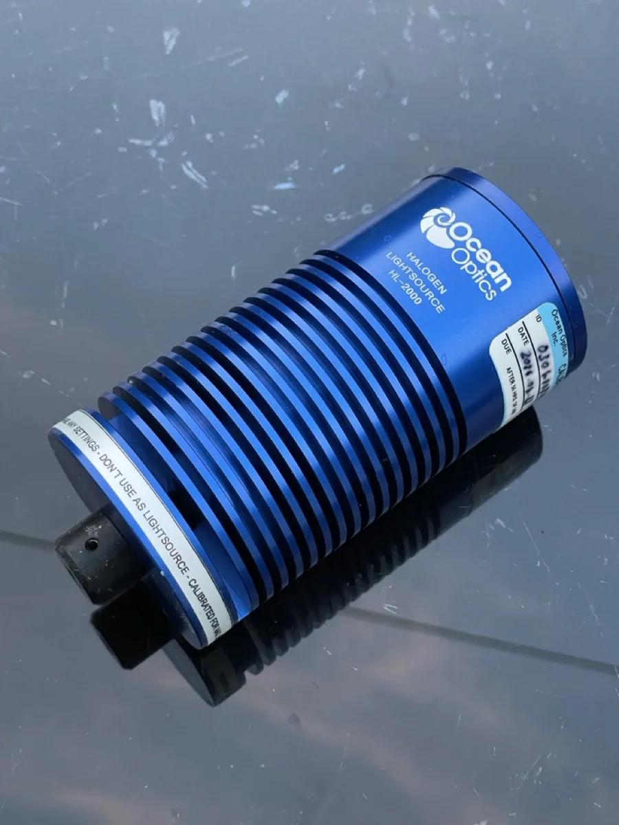
Inside is a tungsten-halogen lamp with a precisely measured emission spectrum. Every unit has its spectral power measured at the factory and ships with an individual calibration certificate traceable to NIST standards.
The lamp is rated for 50 hours of operation, after which the lamp itself has to be recalibrated and recertified. According to the manual, one procedure takes 30 minutes of warm-up and 10 seconds of actual calibration, which means the reference source lasts for roughly 100 calibrations.
It is precisely this calibration against a NIST-traceable standard that gives the measurements metrological weight: this is not "the instrument showed something", but a value tied to a national standard. That is why every measurement on our YouTube channel is made with certified laboratory equipment, not with a pocket spectrophotometer off a marketplace.
OpticalWave — our own software in Python
The second half of the job is how the light is distributed in space. And here we use software I wrote myself, in the spring of 2026.
It all started when OceanView 2, the old program I had bought years ago, refused to launch on a new Mac. After reading around, I realised I would have to buy it again, or try to talk them into a discount on the grounds of a change of computer.
That alone would have been tolerable, but in ten years exactly one update had come out, and on a modern screen it looked as though I were back in the 2000s. All right then, I thought, and decided to read up on how data actually comes out of a spectrometer. And here I was surprised: it turned out to be remarkably simple.
It turns out the spectrometer simply streams data continuously in packets of a certain format, and those packets can be received with an existing Python library. When I managed to receive the first packets I was delighted — all that remained was to process them mathematically.
From that moment began the long and painstaking work on the program I dubbed OpticalWave. Imagination knows no bounds, so I wanted to build the things I had been missing all along, plus add something new that nobody else has. That is how the idea of semi-automatic 2D light maps was born, and later 3D maps as well.
The OpticalWave interface
OpticalWave is software by SPECLED.COM, written entirely in Python for Ocean Optics STS series spectrometers. It controls spectrum acquisition, applies the radiometric calibration and computes the photometric and photobiological parameters of light sources across the 380–800 nm range.
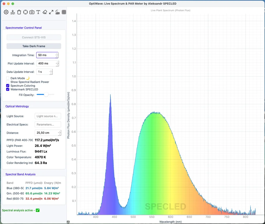
As the screenshot shows, the main window displays the quantum spectrum and the key parameters: PPFD, irradiance, illuminance in lux↗, correlated colour temperature and the colour rendering index. Below that is the spectrum split into three sections: 380–500 nm, 500–600 nm and 600–750 nm — effectively the whole ePAR range.
If needed, the energy spectrum can also be displayed in a separate window.
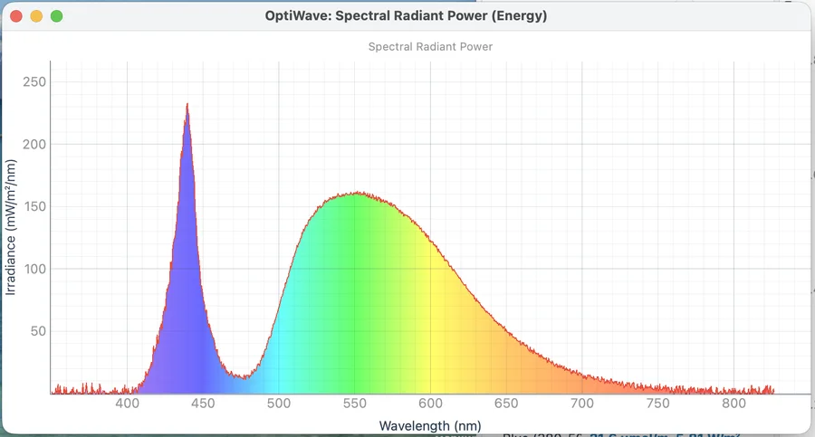
Now that there are two screenshots, you can compare two spectra of one and the same LED on a single page and see the substantial difference between them. For plants, the correct spectrum is the quantum one. Showing an energy spectrum for a grow light is wrong: the quantum spectrum always differs significantly.
How we build light maps for grow lights
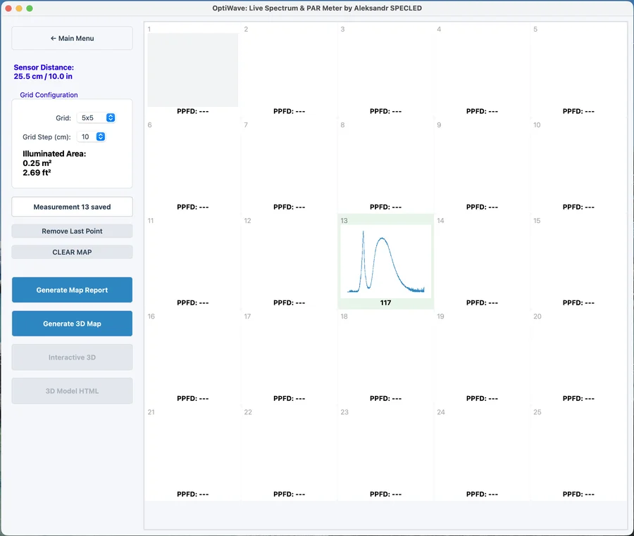
To make 2D and 3D maps easier to produce, I designed a template in which you can set the grid size and the number of cells. The idea is to move the spectrometer across pre-marked cells beneath the lamp while, in the program, you simply click the corresponding cell. The program automatically captures the spectrum and PPFD, recording the data separately for each cell and assembling an array of data.
The 2D light map and the grow light spec sheet
Once I had the template set up for producing light maps comfortably, I built a 2D map generator that outputs a full spec sheet for a grow light. The picture below is an example of what it looks like: this is a test measurement, taken with a phone's flashlight.
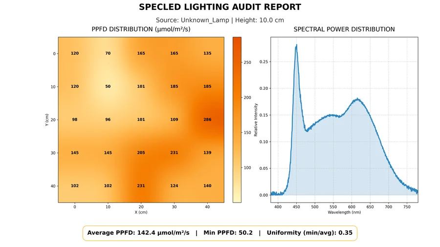
A 2D map answers the question of how evenly the space in a grow tent is lit. It is a top-down view of the area: colour shows how many photons arrive at each point. Hot spots under the centre and dips are immediately visible. Since this is not just a map but also a spec sheet for the lamp, the report states the lamp name (currently Unknown_Lamp), the measurement distance (just 10 cm for now) and the following important parameters:
- Average — the average PPFD across the area, calculated automatically.
- Min PPFD — the minimum PPFD on the light map in question.
- Uniformity — the uniformity coefficient of the lit area, from 0 to 1, calculated automatically. 1 means perfectly uniform; the closer to zero, the worse, as in the example.
The 3D light map
Now for the map in 3D. Its main advantage is that it is interactive and can be rotated right in the browser. In essence it is the same thing as the 2D map, only the peaks and troughs of illumination are shown as ridges and hollows.
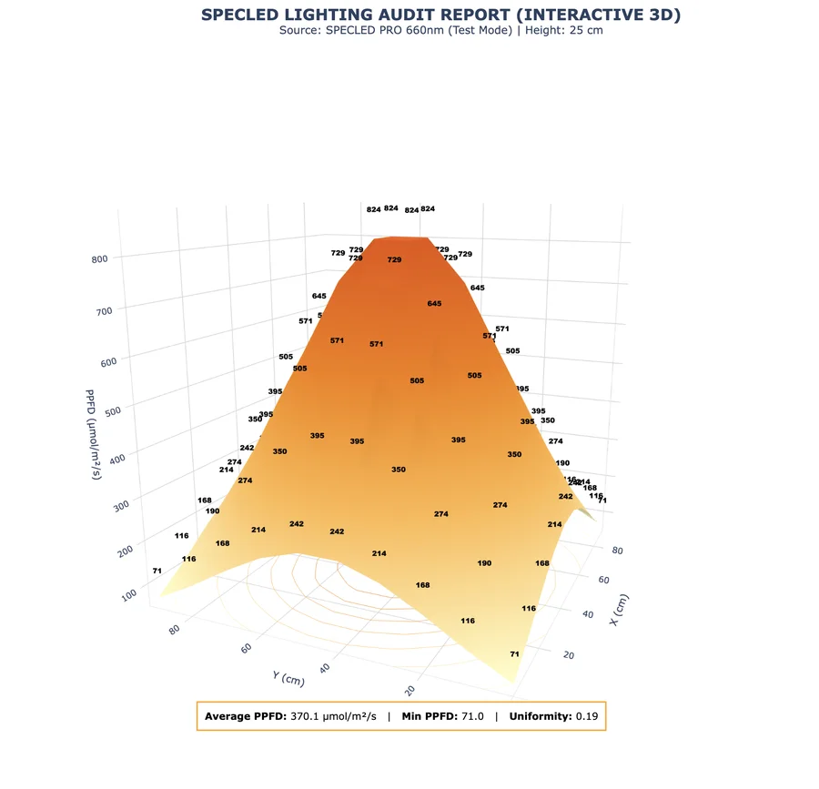
The image shows the light map of an LED flashlight. Clearly there is a maximum in the centre and a falloff towards the edges. The 3D map shows the same thing as the 2D one, only as a surface.
A 3D map makes it easier to judge the character of the falloff: whether it is gentle or abrupt. The overall picture across the area becomes clearer, and these maps are interactive — you can rotate them and look from directly underneath, which is rather fun. I plan to produce maps like these for every grow light in the catalogue↗ and for every LED module for plant lighting↗. A spectrum and a luminance map are a perfect symbiosis. A lamp with a perfect spectrum but a dip in PPFD at the edges will produce an uneven harvest: some plants will simply not receive enough light, and no amount of pretty peaks on the graph will correct this. The opposite situation is no better: a perfectly smooth map with a crooked spectrum means you've uniformly illuminated the area with the wrong light. That's why we measure both to get a complete set of characteristics for a phytolamps or LED modules for plants.
Our spectrum measurement services for grow lights and LEDs
We measure the spectrum and key parameters of phytolamps and other light sources, including individual LEDs and LED arrays. This could be your own assembly that needs testing, or a commercial lamp whose performance you don't trust.
As a result, you receive a quantum spectrum broken down by range, PPFD with calibrated absolute values, correlated color temperature and color rendering index, and, if necessary, a 2D illuminance map with uniformity coefficient and a lamp data sheet. Measurements are performed on NIST-calibrated equipment, and we send the report electronically.
To discuss the project and deadlines, please contact us via the contact form on our website↗.